Making shaded relief from digital elevation models (DEMs) in QGIS

Updated, April, 2021

Tom Patterson, creator of the fabulous shadedrelief.com website, once said, “There is no more important component of a map than the shaded relief.” Who would not agree?

But the topic of creating your own shaded relief from a DEM is rather complex, so I’ve made a few assumptions in this how-to. I’m assuming:

• you know your way around QGIS (I am using QGIS 3.16 for this post)
• you’re familiar with the idea of projections, and re-projecting raster data
• you know that each projection/datum combination has an EPSG number, which is a convenient way to refer to it. For example
  • Lat/Long/WGS84 = 4326
  • UTM Zone 9N/WGS84 = 32609
  • BC Albers = 3005

If that’s the case, there are really only three things you need to know in order to made your own hillshades:  where to get the data, how to transform it, and what pitfalls to avoid.

Why even make your own hillshade?

Usually when I want to include shaded relief in a map that is in British Columbia, the first place I will turn is the WMS service at openmaps.gov.bc.ca: http://openmaps.gov.bc.ca/imagex/ecw_wms.dll?

• 

  The 315 black-and-white hillshade from openmaps.gov.bc.ca. The black-and-white hillshade with the sun at an azimuth of 315° is typically the most useful of the layers on this WMS server.

It’s got some limitations:

• there are only two sun azimuths to select from: 315° (northwest) and 225° (southwest). More flexibility would be good, because each landscape seems to have a different ideal azimuth to bring out the landforms that you want to bring out. More about this down below.
• there’s no height exaggeration possible
• occasionally there are odd artifacts, like straight lines running across the hillshade

On the other hand, you can adjust its brightness and contrast, and use the Multiply blend mode, which means you can do some nice things with it.

• 

  When you set the blend mode of a hillshade to MULTIPLY, it shows through upper layers.

But, if you want to adjust the azimuth or exaggerate height, you’ll need to find a DEM and make your own hillshade.  It’s well-established (though not well-explained) that the human eye needs to see light from above, preferably from above and to the left. If your map is, say,  south-up, you will need a hillshade where the light comes from the southeast (which will be in the upper left).

• 

  Now south is at the top (map is rotated 180°) and the shaded relief appears flat or inverted. For this map you would need a hillshade where the sun’s azimuth is southeast, or 135°.

• 

  Here the map is still rotated 180°, but the hillshade has been manufactured with an azimuth of 135°. The mountains look like mountains again.

• 

  A 3x vertical exaggeration of the terrain emphasizes the detail in the valley bottoms.

The overall process

• 

Let’s talk about the three principles.

1. The hillshading algorithm requires a DEM in a metric projection. That means that DEMs projected in degrees won’t work: you have to re-project them first. [Although maybe sometimes not.] Unfortunately, just about all DEMs come projected in degrees, so re-projection is a must. (The Geospatial data extraction site at canada.ca, however, is one that does offer DEMs projected in metres. Choose to download your data in the “Canada Atlas Lambert (EPSG: 3979)” projection.)
2. The scale of your final map determines what sort of cell size you want in your re-projected DEM. A DEM with 10m cells is far too detailed for a map at 1:500,000, and the file would be enormous. On the other hand, a cell size of 500m would make a very coarse hillshade at 1:500,000. As a general guideline, divide the denominator of your scale by 3,000 (for screen display) or 10,000 (for printing at 300dpi) to get roughly what cell size you want. So if your map is 1:100,000, and it will be printed at 300dpi, you’d be looking for a DEM with (roughly) 10m cells.
3. In QGIS it is an option to style any DEM as “Hillshade” (other options are singleband grey, multiband colour, paletted, singleband pseudocolour, etc.) but the GDAL hillshading algorithm in the toolbox (Processing>Toolbox) produces a better result.

Acquiring DEM data

The first thing you need to do is pick your resolution. Because DEMs usually come projected in 4326, DEM resolution is typically expressed in arc-seconds, or seconds of latitude. Because degrees of latitude in Canada are bigger than degrees of longitude, these cells are not square on the ground. They are rectangles that are taller (north–south) than they are wide (east–west).

What you want to know is how these non-square cells measured in arc-seconds will convert to square cells measured in metres. Here are some rough ideas.

Resolution (degrees)	Resolution (metres)	Source	Limitations	Recommended scale (screen/print)	Notes
0.75″ or 0.0002083333333°	20	CDEM or CDSM at https://maps.canada.ca/czs/index-en.html	Canada only	1:60,000/1:200,000	Alternately, can be downloaded in a metric projection
1″ or 0.0002777777°	30	SRTM1 at https://dwtkns.com/srtm30m/	60° South to 60° North	1:90,000/1:300,000	Comes in 1° x 1° tiles
3″ or 0.000833333°	90	SRTM3 at https://dwtkns.com/srtm/	60° South to 60° North	1:270,000/1:900,000	Comes in 5° x 5° tiles
15″ or 0.00416667°	450	SRTM15+ at https://topex.ucsd.edu/WWW_html/srtm15_plus.html		1:1,300,000/1:4,500,000	The world is divided into 33 tiles.

From here, I’ll demonstrate how this works with an actual example. In this case I want shaded relief for a series of maps that are all in the same area, and range in scale from 1:45,000 to 1:130,000. Looking at the chart above, this scale range suggests I can get away with using SRTM1.

• 

  Displaying an area in a print composer with grid of lines in CRS 4326 is one way to figure out which tiles you’ll need.

So I go to Derek Watkins’s 30-Meter SRTM Elevation Data Downloader, and select each of those SRTM1 tiles.

• 

  Downloading DEM tiles from Recordlist

Once they are downloaded and unzipped, I’ll read them into QGIS to confirm that they cover the right area.

Merge and Clip

You will want to merge all of the individual DEMs into one, using Raster>Miscellaneous>Merge. (Incidentally, they do not have to be read into QGIS to do this.) If you made shaded relief out of each individually, there would be some artifacts along the lines where tiles meet.

• 

  QGIS’s raster merge dialogue

I tend to name the resulting merged DEM with “_4326” on the end so that later I will know what projection it’s in.

It’s tempting to display as hillshade now, but don’t. The hillshade styling is not meant for DEMs projected in degrees.

• 

  Styling the DEM as “hillshade” produces ugly results when the DEM is projected in degrees

If you want to clip the merged DEM, now is the time to do it. Remember that with Raster>Extraction>Clipper you will need to change the QGIS projection to the DEM’s native projection (4326) before you draw the clipping box. Be sure to check, once you come back to your map’s projection, that the clip you made covers your whole print composer.

Re-project and re-sample

Reprojection is the process of giving raster cells coordinates in a new projection. Resampling, on the other hand, is the process of changing the resolution of the DEM. The two are essentially inseparable, since as you reproject from 4326 to, say, 32609, you will also want to go from the rectangular cells of the degree-projected DEM to nice square cells in the UTM projection.

The first thing to do is to right-click the DEM and choose Save As… so you can see the dimensions of the original DEM cells.

Note that once you set the CRS for the saved copy to be 32609, you get a suggested resolution of (roughly) 17 x 31m cells. That’s the native cell size of this SRTM DEM at this latitude. Note down the “17” (the smaller dimension)  somewhere, and close this dialogue.

You can reproject and resample using QGIS’s Save As… feature, but you don’t get control over the resampling algorithm used, and the results, once you get to the final hillshade, are ugly.

• 

  When you reproject using Save As…, the final hillshade sometimes has these weird cross-hatching artifacts in it

Instead, you want to re-project and re-sample with the Warp tool in the toolbox. (Go Processing>Toolbox and search on “warp.”)

• 

  The toolbox’s Warp tool

In this dialogue…

• Source SRS should be 4326
• Destination SRS should be 32609 (or whatever metric projection you are making your final map in)
• Output file resolution can be whatever you want, but I get good results with the smaller of the two cell dimensions I saw in the Save As dialogue — in this case, 17.
• Trial and error with making hillshades has convinced me that the best resampling method to choose here is “bilinear.”
• I name the resulting DEM with a “_32609” on the end so I will know its projection in the future.

The new 32609 DEM should look the same as the 4326 DEM when read into QGIS, but if you go to the Metadata tab in Layer Properties you’ll see it has a cell size of 17 metres, and quite different pixel dimensions.

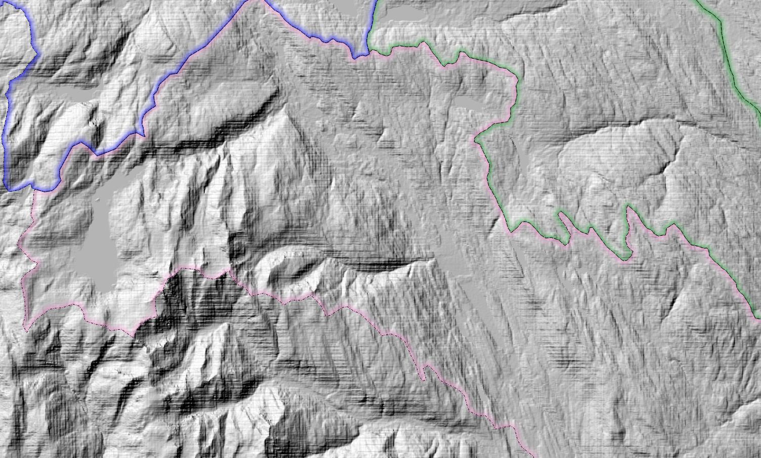
For your final hillshade, the one you use in your map, you will want something better that what you get if you just style this DEM as “hillshade.”  But for now, go ahead and style it as “hillshade.” This enables you to play with the sun azimuth and elevation, and the vertical exaggeration, to see what is going to work best for your terrain. The human eye probably wants an azimuth around north-northwest (337.5) but there are a lot of azimuths on either side that will work.

Notice how changing azimuth changes what’s brought out in this piece of terrain:

• 

• 

• 

Make a static hillshade

Now if this DEM-displayed-as-hillshade has no strange artifacts, you’re done. But if you want a smoother results, it’s time to take the azimuth, sun elevation and vertical exaggeration you’ve chosen, and go over to the GDAL Hillshade tool in the toolbox. (Go Processing>Toolbox and search on “hillshade.” Notice that two different hillshade tools are available: a QGIS one, and a GDAL one. The GDAL one has an interface I prefer.)

Enter your vertical exaggeration under Z factor, your sun azimuth under Azimuth of the light, and sun elevation under Altitude of the light. Generally speaking you leave scale as 1.0000, because your have re-projected your DEM and the vertical units and the horizontal units are both metres.

• 

  The toolbox’s Hillshade tool

And here’s the result

• 

  Look, no artifacts!

Displaying hillshades

Hillshaded made by GDAL tend to be a bit darker than we want. Their raster values run from 1 to 255, and by default this gets displayed as a singleband greyscale from pure black to pure white. But you probably don’t want pure black areas in your map, or at least not very many. Areas of solid black can’t have much information in them.

• 

Hillsahde as greyscale where raster values from 1 to 255 are mapped to pure black to pure white

Two common solutions are to adjust the opacity of your hillshade, or to increase its brightness.

• 

50% opacity

• 

Brightness +80, contrast -35

A solution that I like is to build a colour ramp that runs from 50% grey (#808080) to white (#ffffff),

• 

and then display the hillshade as singleband pseudocolour, using this colour ramp.

• 

What I like about this is that I then know that no part of my hillshade is darker than 50% grey.

Typically you combine the hillshade with the other layers of your map by assigning it a Blending mode of Multiply.

• 

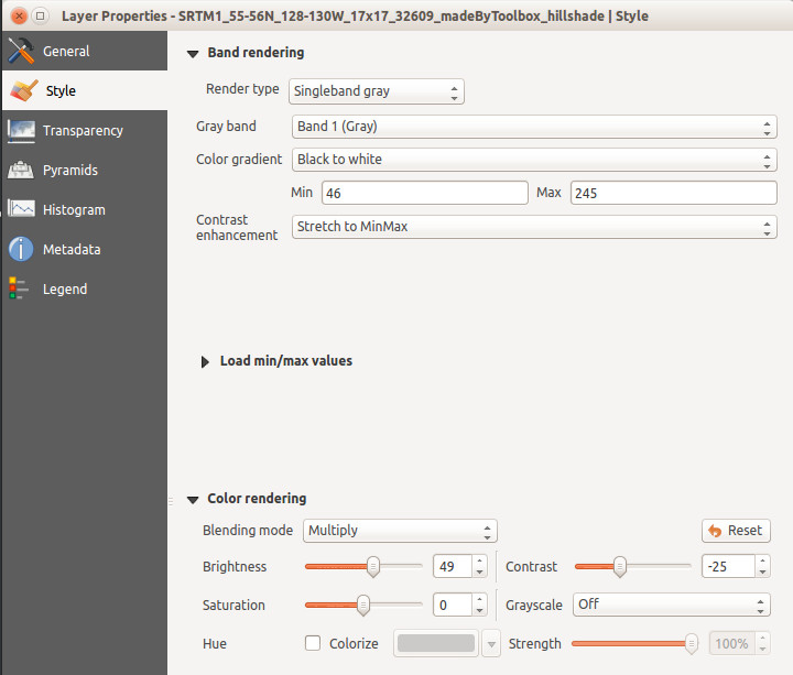
  Multiply causes the values (lightness, darkness) in the hillshade to be applied to layers above and below it.

So you can get something like this.

• 

  Overlaying a hillshade whose blend mode is set to Multiply

Be aware that if you have other layers in your stack that have partial opacity, it does make a difference whether your hillshade is above or below them. In general you get the most predictable results by using a Blending mode of Multiply and placing the hillshade at the top of your stack.

That’s it. Using these techniques, you should be able to manufacture hillshades with any azimuth, pretty much all over the world. It gets the most challenging when you are mapping at large scales like 1:20,000.

Finally, if you master this, and you are really in love with shaded relief, you will want to experiment with making shaded relief in Blender.