Shaded relief with BlenderGIS, part 2

With the DEM read in, we’re now ready to adjust the many parameters in Blender which determine what we’ll get. Here again is the overall procedure (mentioned in the previous post) . We’re now at step 5.

1. Select the Cycles Renderer
2. Read in the DEM as DEM
3. Create new material
4. Adjust Z scaling
5. Create and adjust the georef camera
6. Correct final pixel dimensions to match the input DEM
7. Adjust lamp location and properties
8. Test render
9. Adjust final parameters
10. Render

Create and adjust the georef camera

With the plane selected, go to the the (new) GIS tab on the left, and, under BlenderGIS, click Georender.

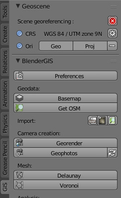
This creates a camera at an appropriate distance above the plane. It will appear in the tree of objects (upper right) as “Georef cam”. It has been placed high enough (Z value of 16791) that it is above the highest point on the plane surface. Note that it is important to have set your Z scaling before creating the Georef cam.

If you look at the camera’s Object Data>Lens, you’ll see that BlenderGIS has automatically set it to Orthographic. It’s a good idea to note the camera’s clipping Start and End, because you may have to adjust these later.

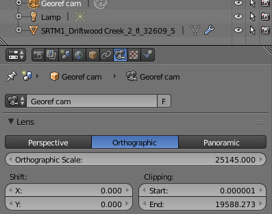
As well, if you check out the Scene’s Scene panel, you will see that the current camera has been set to this new Georef cam.

Correct final pixel dimensions to match the input DEM

If you go to the Render tab, under Dimensions>Resolution you can see the pixel dimensions of the final image as suggested by BlenderGIS. In this case, as I noted before, one cell has been dropped in each dimension, so it is 5029 x 3276.

I correct these to the actual values (5030 x 3277, in this case) so that the dimensions of my final image match the DEM. That way I can pair the TFW world file with the image created by Blender, and read it into QGIS georeferenced.

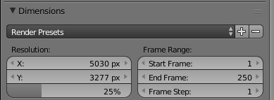
While I’m at it, I’ll set the Resolution percentage to 25%. This way I can get a test image without doing a full render. While I’m here on the Render tab, I’ll go to the Light Paths panel and set it to Limited Global Illumination. Now we’ll check that all elevations in the DEM are visible to the camera. Pop into Camera Ortho view (Numpad 0 while the mouse is over the 3D View). You are looking for  black faces where the higher parts of the DEM have been cut off. It can look something like this: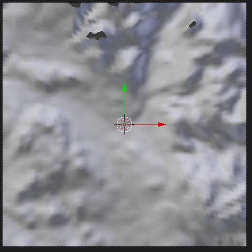BlenderGIS was updated in December 2014 to place the Georef Cam high enough so that this typically does not happen (Thanks!), but I’ll still discuss what to do in case you do encounter it. This could happen if you, say,

• create the Georef cam before you increase Z scaling on the DEM.
• create the Georef cam at a time when the View number in the Subsurf modifier is low (e.g., 6). In this case the displacement is quite generalized; the Georef cam will be placed high enough to clear it, but not the actual high points that pop out when you render at 11.

What’s happening here is that the camera only “sees” objects that fall between the Start and End clip distances we noted a few steps back. The Start and End are measured from the camera outward (or down, in this case).

Specifically, in the image above, I had a camera at 11,706m, with a Clip Start of 0.5 m, and a Clip End of 8011.5 m. If you do the math, you’ll see that this means that the maximum elevation at which it can see objects is 11,705.5 (that’s 11,706 – 0.5). The minimum elevation at which it can see objects is 3694.5 (that’s 11,706 – 8011.5).  Our DEM originally contained elevations from 739 to 2379, but now we’ve scaled it up 5 times, so its minimum is 3695 (= 739 x 5) and its maximum is 11,895 (= 2379 x 5).  The black patches are the elevations that are higher than 11,705.5 m.

If I do a test render with these settings I’ll get the image below; I’ve circled the black patches where the highest peaks were cut off.

In this case we need to raise the camera to just above the max value in the DEM, and then adjust the Clip Start and End distances to encompass the whole DEM. Since the DEM ranges from 3695 to 11,895, let’s put the camera at 11, 896, leave Start at 0.5, and set End to 8201.5.

 Adjust lamp location and properties

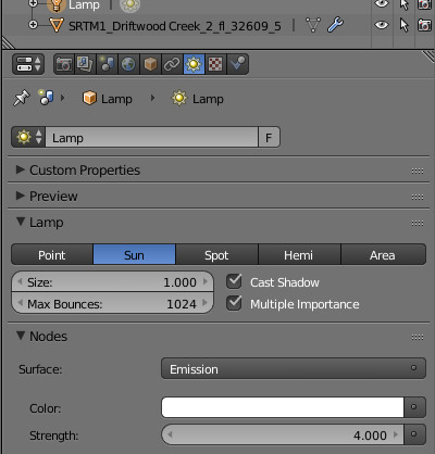
This does not differ in any way from what you would do with the Subdivide method. Set the Lamp to Sun, and click Use Nodes. I like a sun size of 1, Cast Shadows checked, and a Strength of 4.

Then change to the Lamp’s Object tab, Transform section, and set its X, Y and Z Rotation. In this case I want an elevation of 40°and an azimuth of 337.5°, so I choose X=0, Y=40, and Z=112.5. Remember that Blender measures the sun azimuth counterclockwise from East.

 Test Render

Hit F12 to see a test render at 25%. It should look grainy but basically correct.

Final adjustments

At this point you can play with:

• lamp rotation, strength, size
• Z scaling on the model
• the Render number under the Subsurf modifier on your plane

When you’re ready to go,

• On the  Render tab>Dimensions, raise the Resolution from 25% to 100%
• On the  Render tab>Sampling set the Samples Render number to 200. This high sampling number makes the rendering process take a long time, but it’s worth it. Check out this comparison of the same scene rendered with sampling 200 (left) vs sampling 90 (right):

  

  Note the noise in the shadows when sampling only 90 times (right image) as opposed to 200 times (left image).

• On the Render tab>Output, set the image type to TIFF (if you want to pair it with a pre-existing TFW after you render)
• Save your session to a .blend file using File>Save As…

Render

Two options here. One is that you can hit F12 and go out for coffee.  When it’s done, hit F3 to save.  Or, you can close Blender and render that .blend file you just saved from the command line. This saves the GUI rendering, and so it takes less time — you might get 10-40% off the regular render time.

Let’s say your  .blend file is called tile_4_4.blend. The command line to render it would be

/path/to/blender -b tile_4_4.blend -o hillshade_4_4.tif -F TIFF -f 1

The switches are:

-b     run in background (no-GUI) mode

-o     the output filename

-f 1    render just one frame.

Pulling the result back into QGIS

Let’s say you have saved the rendered image as hillshade.tif. Rename a copy of the world file you created way back at the beginning to hillshade.tfw.

QGIS should be happy to read in hillshade.tif now as raster data, although it will probably ask for the CRS. (You know the CRS because you specified it when you re-projected the DEM, and when you read it into Blender.)

It works quite well in QGIS to set the Blend Mode of the hillshade to Multiply, and then overlay it with layers representing vegetation or elevation.

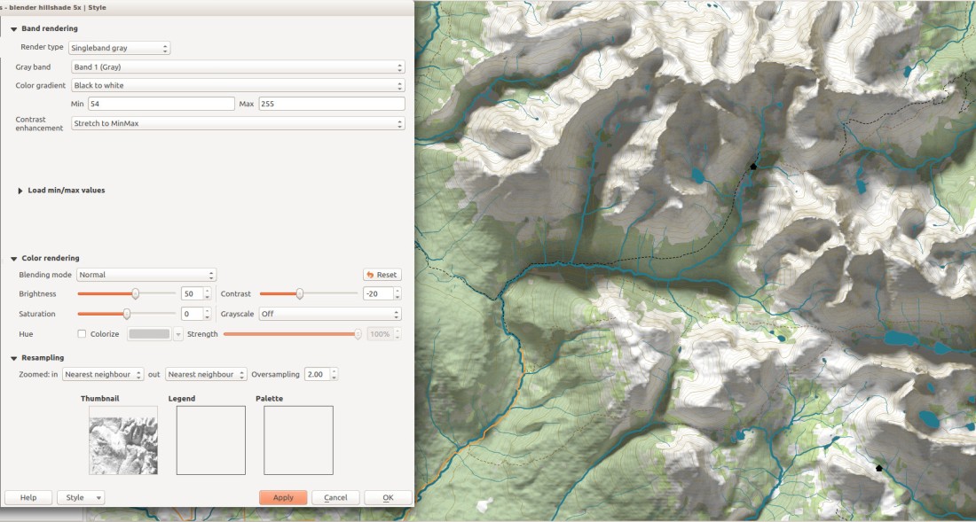
The shadows can be thunderingly deep in these hillshades…

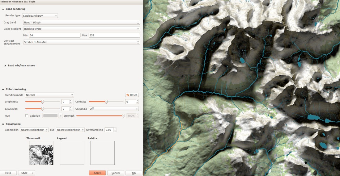
…so it can be good to display them with increased brightness and decreased contrast.