Shaded relief with BlenderGIS, part 1

Note: This tutorial has now been superseded by a new one which uses Blender 2.8.

[The BlenderGIS add-on has now been improved to the point where generating shaded relief is downright easy. So, I have updated this post (April 2017) to reflect how one uses its latest version. Also the latest version of Blender (2.78c).

You may have read Daniel Huffman’s great tutorial about created shaded relief using the free, open-source animation software, Blender. This is an update of Daniel’s video tutorial for his method.

In Daniel’s method, you subdivide a plane to create a grid of finely spaced points. You then apply a Displace modifier to the plane with a DEM, and get some very realistic results.

There are a few things about this method, which I’ll call the Subdivide method, that were difficult for me. For one thing my meager 4GB of RAM precluded subdividing the plane more than about 1500 times. So I went searching around, and found to my surprise that there’s a plug-in available for Blender called BlenderGIS that does much the same thing. But unlike the Subdivide method, BlenderGIS uses a Subsurf modifier. This saves a lot of memory.

Note that distinction: subdivide vs. subsurf. That’s important

As well, BlenderGIS offers a few interesting tools for the GIS user. One is the ability to create a GeoRef camera, correctly configured and positioned to shoot an image of your lit DEM. Another, which I haven’t really explored, is the ability to read in shapefiles to add features to the DEM surface.

In this series of posts I give a tutorial for how to use Blender GIS’s subsurf method to achieve results similar to those obtained with the subdivide method.

I’ll assume that you have watched Daniel’s tutorial, so finding your way around Blender for purposes of generating a shaded relief isn’t too hard for you; and this of course implies, as well, that you are the kind of GIS user who knows what a DEM is. My workflow mostly happens under Ubuntu 14.04 using QGIS and GDAL tools.

We’ll do this in two parts. Part 1 is about installing Blender GIS,  preparing your DEM, reading it in and adjusting the vertical exaggeration. Part 2 is about creating the georef camera, placing the lamp and adjusting some final parameters.

Installation of BlenderGIS

The master instructions are in the BlenderGIS wiki at https://github.com/domlysz/BlenderGIS/wiki/Install-and-usage  However, I will paraphrase them here.

Go to the BlenderGIS site on github and hit the Clone or Download button. You will receive a .zip file, which you can store pretty much anywhere.

Within Blender,  at File>User Preferences, the Addons tab, click Install From File, and point it at the .zip file you just downloaded. (You don’t have to unzip it.)

Once its installed, you still have to do two things:

1. Check the box next to 3D view: BlenderGIS to enable it
2. Click Save User Settings

That’s it. BlenderGIS is installed.

Preparing your DEM

I used to use divide my DEM up into square tiles, and feed these one by one through Blender. However BlenderGIS in no way requires this.

Projection and resolution

BlenderGIS claims that it can now read a DEM projected in “WGS84 latlon”, but I have not had very good results with this. I still prefer a DEM that is in a projection that uses metres. Typically for me this would be a UTM projection.

You may also want to re-sample your DEM, so the cell size is appropriate to the scale of the map you are making.  I use this guideline: the DEM resolution should be map’s [metric] scale divided by 10,000. For example, if the map scale will be 1:100,000, I want a DEM with 10 metre cells. For a 1:30,000 scale map, I want a 3 metre DEM. It’s just a general guideline.

Before you re-sample and re-project, however, be sure to float your DEM and create a world file.

Float DEM

Most DEMs come as integer values. Floating it means converting it to a DEM that can has floating point elevation values.  You can do that with a line like this with gdal_translate.

gdal_translate -ot Float32 myDEM.tif myFloatDEM.tif

where the -ot switch specifies output type.

World file

You’ll need the world file when you are done, to georeference your hillshade.

Almost all DEMs come as GeoTiff files, and the corresponding world file extension is .tfw. An easy way to create a TFW World file is with the GDAL command gdalwarp:

gdalwarp -co "TFW=YES" myGeoTiff.tif deleteme.tif

This just makes a second copy of myGeoTiff.tif called deleteme.tif, but in doing so it creates a world file called deleteme.tfw. (The switch -co “TFW=YES” means to use the creation option “TFW=YES.”) The world file is what you really want, so delete the deleteme.tif. The world file and the main image file need to share the same name, so rename the TFW to myGeoTiff.tfw.

Re-sample and re-project

I like to do these two operations simultaneously with gdalwarp. In the following example, I am re-projecting out of 4326 (the EPSG code for lat/long/WGS84) into 32609 (the EPSG code for UTM Zone 9 north/WGS84).

Where

-s_srs

the Spatial Reference System (projection & datum) of the original

-t_srs

the SRS of the result

-r

resampling method

-tr

resolution, in metres

-of

output format

gdalwarp  -s_srs EPSG:4326 -t_srs EPSG:32609 -r bilinear -tr 5 5 -of GTiff myFloatDEM.tif myFloatDEM_32609_5x5.tif

Note that the terms “projection/datum”, SRS (Spatial Reference System) and CRS (Coordinate Reference System) are interchangeable for our purposes.

Now we’re reading to open up Blender and get started.

Overall process

The process will essentially go like this (and you can use this as a checklist once you get familiar with it):

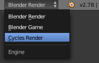
1. Select the Cycles Renderer
2. Read in the DEM as DEM
3. Create new material
4. Adjust Z scaling
5. Create and adjust the georef camera
6. Correct final pixel dimensions to match the input DEM
7. Adjust lamp location and properties
8. Test render
9. Adjust final parameters
10. Render

The green steps are probably already familiar to you from Daniel’s tutorial.

Select the Cycles Renderer

Open up Blender and delete the default cube that appears. Switch the selected renderer to the Cycles Renderer.

Reading the DEM in

File>Import> Georeferenced raster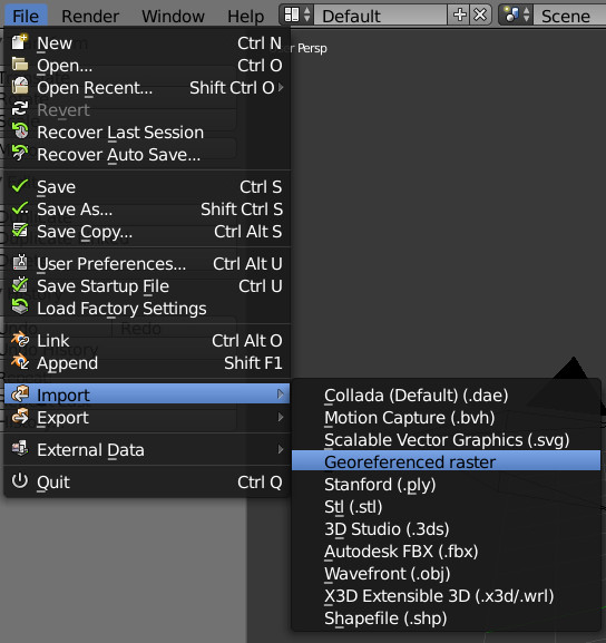

Select your floated, re-projected, re-sampled DEM, and in the left margin, where it says Import georaster, set Mode to As DEM, Subdivision as Subsurf, and select the correct CRS for your DEM.

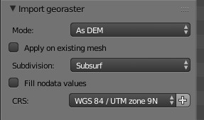
If the CRS you want to use is not on the dropdown menu,you can add it by clicking the “+” button, checking the Search box, typing in the EPSG code for your CRS into the Query box, and hitting Enter. It should appear in the Results box, and then you just click OK.

With all these things set, you click Import Georaster, and the result is a somewhat flabby-looking, grey plane.

Tap n (with the cursor over the 3D view) to bring up the 3D view numeric panel, and we’re ready to go for a tour of things that BlenderGIS has done automatically. You don’t ordinarily have to check these things, but they are worth knowing about.

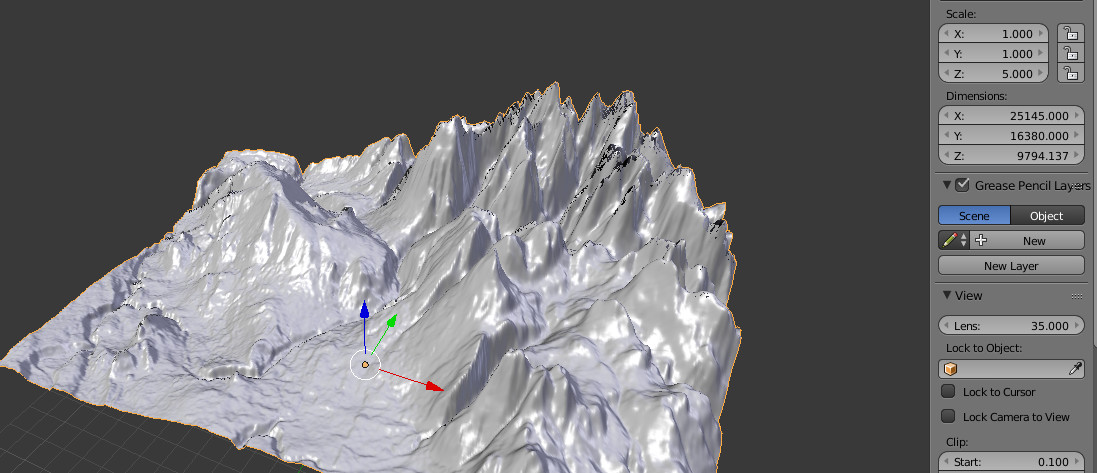
• On the 3D view numeric panel we can see that the dimensions of the plane are the real-world dimensions of the DEM. In this case I’m using a 5030 x 3277 DEM with 5 m cells. For some reason BlenderGIS drops one cell in each dimension, so the DEM is 5029 x 5 on the X dimension (25145), and 3276 x 5 on the Y dimension (16380). metres on a side. We also see the thickness (Z dimension) of the DEM, which is 1911.56 metres.

• Also on the 3D View Numeric Panel, under Display, we can see adjustments to the grid floor. It gives values for Lines and Scale. Ordinarily (e.g., with the default cube) these will be values like 16 lines and a scale of 1. This means lines extend out 16 from the origin and no more, and each square is 1. After BlenderGIS has read in a DEM,  these can be more like 25 lines with a scale of 1000. In this case we have 25 lines on each side of the origin and each represents 1000 units (corresponding to metres).

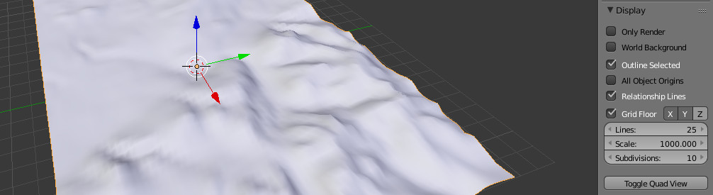
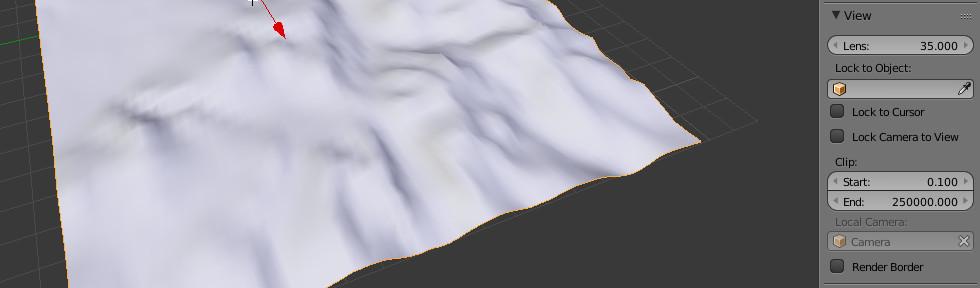
• Again on the 3D View Numeric Panel, under View, the clip distances represent the nearest and farthest you can see the object in perspective view. Ordinarily (e.g., with the default cube) these will be values like 0.1 to 1000. With a DEM read in these can be more like 0.1 to 250,000.

• No longer on the 3D View Numeric Panel, but under Scene>Custom Properties, BlenderGIS has added a crs X and crs Y which correspond to the UTM coordinates of the centre of the plane. This is how the plane can be centred at (0,0), but any additional georeferenced data placed over it will be in the correct place. There’s also an SRID, and even a latitude and longitude.

To understand how the DEM was used to displace a plane, go to the Modifiers tab for the plane. You will see two modifiers have been created. The upper one, called DEM, is a Subdivision Surface, or Subsurf. This kind of modifier subdivides the plane on the fly, and you can specify separate subdivision factors for View mode (what we’re doing right now) and Render mode (when you render the image). The beauty of the Subsurf modifier is that you can leave the View mode number low (e.g., 6) but set the Render number high (e.g., 11).

The factor is used as an exponent of 2, so our View mode is 2^6 or 64 subdivisions along the side of the plane. This is a small number considering that the DEM itself is thousands of points on a side. Which is why the view looks lumpy. 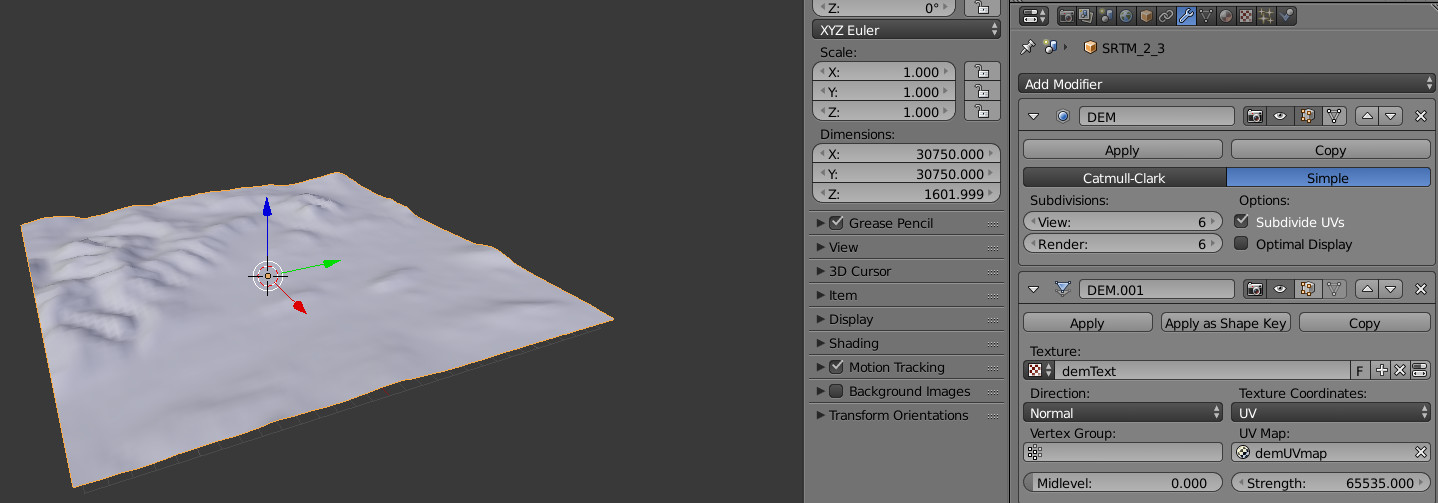The second modifier, called DEM.001, is a Displace modifier, and it applies the DEM to the subdivided plane much as in the Subdivide method.

Try changing the View number on the Subsurf modifier, and watch the fineness of the plane increase. You’ll notice that it takes longer to adjust the 3D view each time you increase the View number by 1, because you are doubling the number of subdivisions. A view number of 6 corresponds to 64,  7 to 128, 8 to 256, 9 to 512, 10 to 1024 and 11 to 2048 subdivisions. 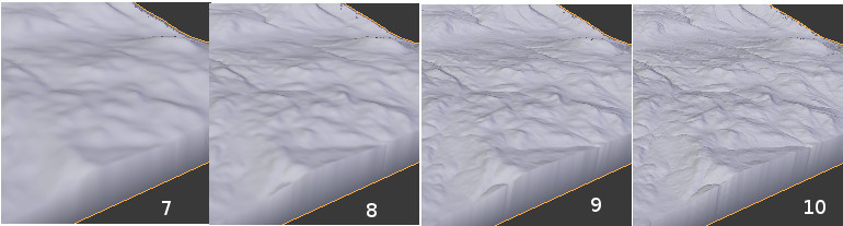By the time you get to 10 or 11, you’ll notice the status bar at the top of Blender is reporting a lot more memory use, 1.2 GB in this case.

Go ahead and set the View number back to 6, but increase the Render number to 10 or 11. Because this higher number of subdivisions will be performed on the fly during render, it takes no memory now.

Create new material

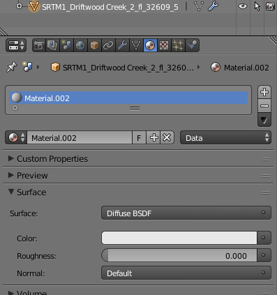
If I now go to the Material panel for the plane, I’ll see that at this point I have no material.

I click New to create a new one. I get the default Diffuse BSDF  material, with a roughness of 0. This is fine, and if I want I can change the material or some of its parameters later.

Adjust Z scaling

Last, we’ll adjust the Z scale factor in the 3D View Numeric Panel to reflect the vertical exaggeration we want. I’ll use 5 in this case. Note that the Z dimension of the plane jumps up to 5 times its previous value, to 9794.137 in this case.

Go on to Part 2.